
Low input or inhibition? Quantitative approaches to detect qPCR inhibitors
Blog

Inhibitors may impact any polymerase chain reaction (PCR) or reverse transcription-PCR (RT-PCR) assay. In a common PCR you can easily see if the product has not been amplified through agarose gel detection. However, the accuracy of qPCR, RT-qPCR, and multiplex-PCR results are essential for many applications. Quantification errors may not be of little practical importance, but they could have substantial consequences in all other situations. Such error may make the difference between up- or down-regulation, affect medical and veterinary decisions, and distort allocation of rare forensic sample to different forensic tests. Additionally, it may determine approval or disapproval of food and water for use, change qualification or disqualification of genetically modified products, and harm many other important decisions, which are based on the measured levels.
qPCR refresher
PCR is a widely used molecular
biology technique to amplify and detect DNA and RNA sequences. Most
applications focus on its utility to turn a small amount of DNA into a larger
amount, necessary for gel electrophoresis and most forms of DNA sequencing, but
it also limits how informative PCR can be. However, quantitative PCR (qPCR)
adds two elements to the standard PCR process: fluorescent dye and fluorometer,
turning the procedure in a measurement technique on its own. The fluorescence
signal increases proportionally to the amount of replicated DNA as PCR
progresses and hence the DNA is quantified during each cycle.
While
running a qPCR, we obtain an amplification plot, which resemble a sigmoidal
curve with three distinct phases: (1) a baseline that gradually
transitions into (2) an exponential region, followed by (3) a plateau, which
indicates that amplification is reducing (Figure 1A). Importantly, a threshold
is placed at the point when the reaction is at the beginning of the exponential
phase, therefore it will not be confused with the background signal. The number
of cycles from which the reaction curve raises above the threshold line or
intersects with it, is our Ct (crossing threshold), Cp (crossing point) or Cq (quantitation
cycle) value. For simplicity, the term “Ct” will be used in this article. The
Ct value indicates how many PCR cycles are required to detect a real
amplification signal and is inversely correlated to input template amount. It means
that if there is abundant template, it takes fewer cycles to amplify and
quantify it. If the sample contains fewer template, the Ct value goes high as
it takes more cycles to progress the reaction.
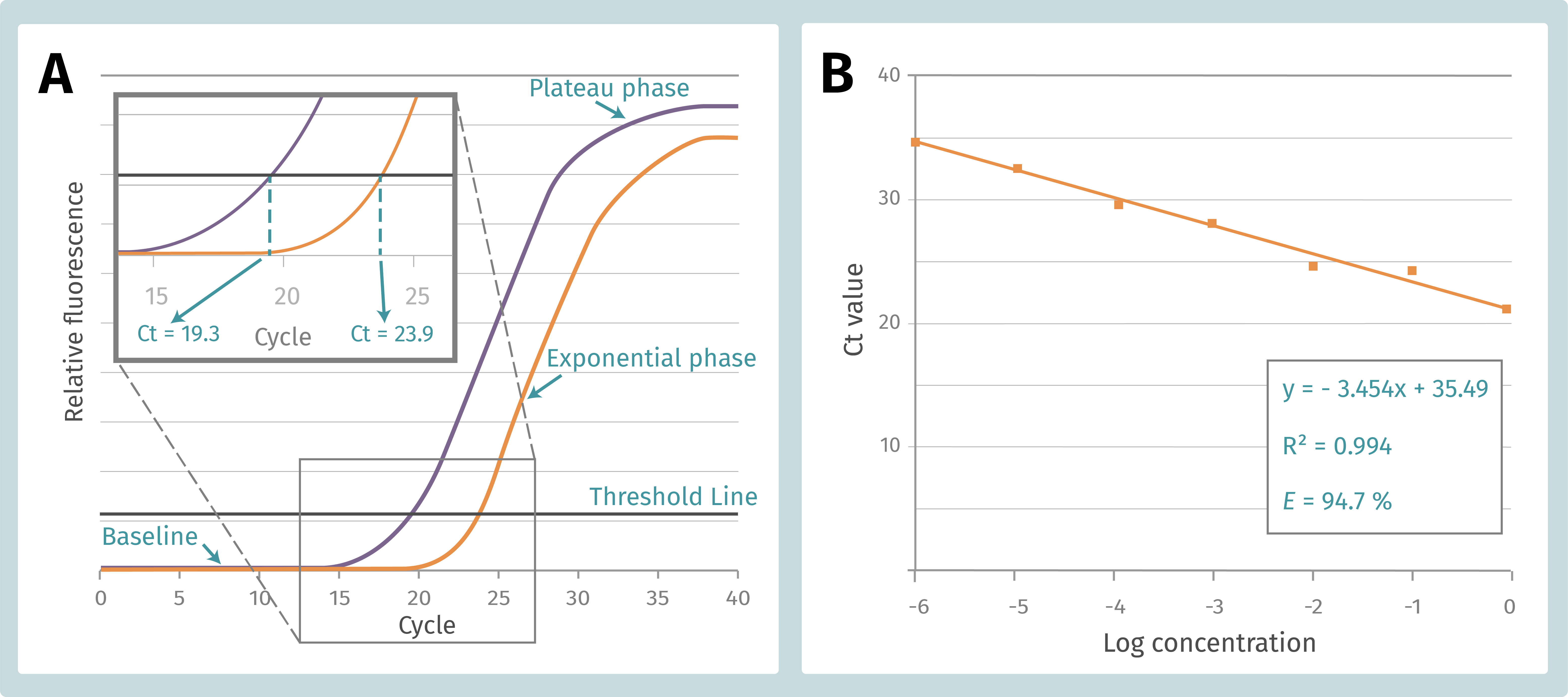
Figure 1. A. qPCR standard curve composition and Ct calculation. B. qPCR efficiency calculation form the standard curve of sample serial dilution.
Why do we review all these concepts? Because high Ct values could be also an indicator of qPCR inhibition. We have talked in our previous article about PCR inhibitors , which can exert it inhibition at different levels. They can: (1) interfere during nucleic acid extraction, (2) degrade template and/or primers, (3) inhibit reverse transcriptase, (4) interfere with primers annealing, (5) inhibit the DNA polymerase or its activity, and (6) interfere with fluorescence. We also discussed some strategies to remove the inhibitors, how to select amplification/RT enzymes with intrinsic resistance to inhibitors, and the use of PCR additives to negate inhibitor effects. But what happened if we do not success eliminating inhibitors or its effects? In practice, inhibitors will flatten the qPCR curves, thus increasing the Ct values. And as mentioned above, quantification errors may not be insignificant, but they can have severe repercussions in some situations and can jeopardize many other important decisions that are based on measured levels.
The question is, how could one discriminate between low copy number template, or an inhibitor being present in our sample? To infer the quality of our input and the qPCR results accuracy, it is essential to perform some assays and controls during or after the procedure. Let’s review some applicable methods.
PCR Kinetics and Efficiency
It is worth mentioning that the efficiency of a qPCR reaction may be negatively affected not only by sample inhibition due to inhibitory compounds but by a combination of a variety of factors. For example, a non-optimal qPCR primer and/or probe design, formation of primer dimers, incorrect sample dilutions, and pipetting errors across the standards and/or samples. The safest recommendation to maximize results accuracy, is to perform a geometric efficiency assessment on all involved assays.
PCR efficiency (E) is defined
as the fraction of double-stranded DNA molecules that is copied at a given
cycle and is calculated from the standard curve of an assay. A standard curve
is created by preparing individual serial dilutions of a control DNA template,
each diluted by a factor of ten. Each serial dilution is used to perform a
separate qPCR reaction. The subsequent Ct values are plotted versus
the logarithm of the target concentrations, and the standard curve is generated
by fitting a linear line to the data points (Figure 1B). E is expressed
in percentage (%) and is calculated form the slope of the standard curve made
of the sample dilution series (E = 10-1/slope -1). For a
10-fold dilution series the efficiency is 100 % when the slope is −3.33. This
follows from the assumption of a perfect doubling of the number of DNA template
molecules in each step of the PCR. Indeed, E = 100 % represents perfect
doubling of all DNA molecules, and 0 % represents no change in reaction
product. A qPCR efficiency ranging from 90 % to 110 % is considered acceptable,
and results obtained out of this range are cause from different factors (Figure
2).
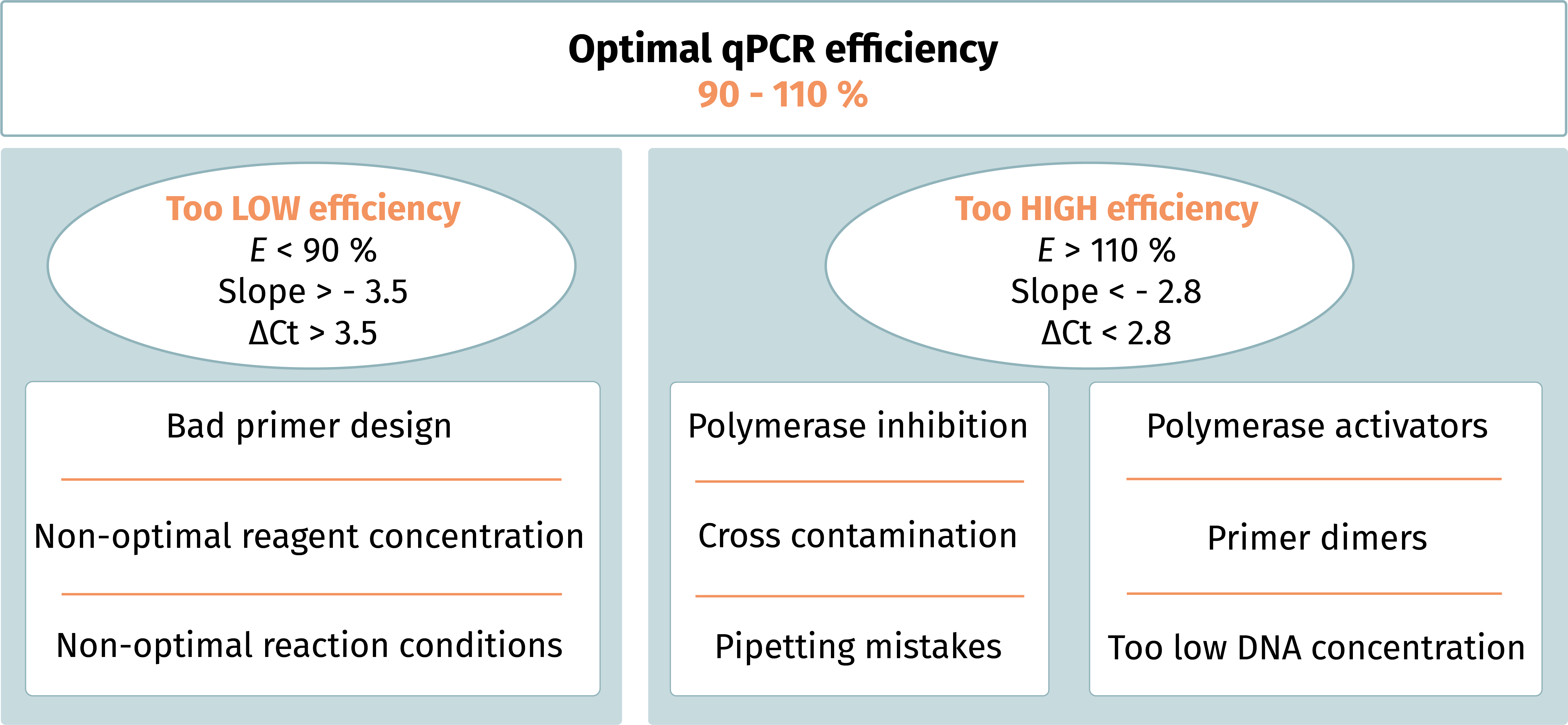
Figure 2. Factors which could determine a non-optimal qPCR efficiency.
Several factors may influence the experiment and thus the standard curve and qPCR efficiency (e.g., laboratory, operator, chemistry, instruments…). We recommend taking in consideration the following aspects1:
- For an optimal primer design, use software tools for control over the design process, such as the control of secondary structures (primer dimers, hairpins), melting temperatures, and GC content.
- Avoid
excessively long standard curves since measurements at extremes may diverge
from linearity and provide misleading estimates of the amplification
efficiency. This is applicable to both high and low target concentrations. For
example, very high target concentrations can have such low Ct value
that base-line subtraction becomes inaccurate.
- To minimize sampling and pipetting errors, utilize as much transfer volume as possible across the dilution steps. We recommend using at least 5 µL transfer volume and generally discourage pipetting volumes less than 2 µL using conventional pipettes.
- To identify the assay linear range and reliably estimate E, we suggest at least five dilution steps, corresponding to 6 different concentrations, if the stock is used as a standard.
- It is preferable to perform a single, highly precise estimation of qPCR efficiency under study conditions that is used for all calculations. It is not advisable to estimate E separately in each experiment run and use it to correct for variation between runs, as this may introduce large imprecision and even systematic bias into measurements that are larger than the inter-run effect, compromising rather than improving data quality.
- The standard curve used to determine amplification efficiency may differ from the standard curve for estimating target quantities in unknown field samples. To assess the performance of the qPCR assay in the absence of interference, the standard curve for qPCR efficiency should be based on a clean matrix. The standard curve, which is used to estimate concentrations of field samples, must be based on representative field matrix to account for inhibition and interference in the field samples.
The qPCR efficiency relates to the value calculated from the slope of a standard curve and relies on the assumption that the amplification curves in the dilution series are parallel at least until reaching the threshold. Hence, for proper quantification these methods assume similar amplification kinetics up to the threshold among compared reactions of the same sequence. If the assumption is not valid, substantial error into quantification can be introduced. An additional drawback is that it is laborious and costly, since a sample must be analyzed multiple times, and is not applicable on samples with small number of molecules, since they cannot be diluted. Also, interfering substances will be diluted as well, and qPCR efficiency will change.
In routine analysis, there are two additional ways to evaluate if the assessment is affected by qPCR inhibition: (1) using amplification controls or (2) investigating amplification kinetics through the actual amplification curves of the target DNA (kinetic outlier detection (KOD)).
Control reaction to assess qPCR inhibition
To determine the inhibitory effect of all substances present in a nucleic acid preparation, we recommend carrying out qPCR control reactions. We can distinguish different types of controls according to the controlled steps (process/preparation control, amplification control) and the implementation of the control reaction (internal or external control). A process control is added at the starting point of sample analysis, e.g., before nucleic acid extraction. Thereby it passes all preparation steps. In contrast, an amplification control is added to the nucleic acid extracted from the sample thus controlling only the performance of the qPCR itself. An internal control is analyzed in the same tube as the target, whereas the external control is analyzed in a separate aliquot of the sample.
The application of internal amplification controls (IAC) is well-established and highly recommended in diagnostics. This method was adopted in 1995, for detection of qPCR inhibition in DNA quantification by the European Standardization Committee (CEN) and the International Organization for Standardization (ISO). IAC is a non-target DNA or RNA spiked-into a test sample at known amount and co-amplified with the target sequence. Following the amplification, the Ct of the IAC is compared to the Ct of the same amount of IAC quantified without the test sample. A difference between the Ct values indicates potential inhibition (Figure 3). Meantime, internal controls can be divided into competitive and non-competitive amplification controls.
- Competitive IAC controls shares primer set with the target sequence but can be distinguished from the target by product length or sequence. One limiting factor of this application may be the concurrent use of primers. The concentration of the IAC must be carefully adjusted to the (unknown) quantity of the target sequence in the samples: too many IAC molecules will consume the primers of the target and will itself inhibit the target sequence amplification. On contrary, if the input of IAC is too little, the target sequence will consume the primers and inhibit the IAC amplification and the control will not correctly reflect the presence of inhibitors.
- In contrast, non-competitive IAC controls are amplified with a different set of primers from the target. The final amount of non-competitive IAC amplicon produced is limited by primers concentrations and does not deplete resources needed by the other reaction. Hence, the amount of IAC added is not critical for proper amplification of the target. However, the sequence dissimilarity between the target and the non-competitive IAC, which makes it so easy to use and popular, may cause it to fail to accurately reflect sequence-dependent inhibition.
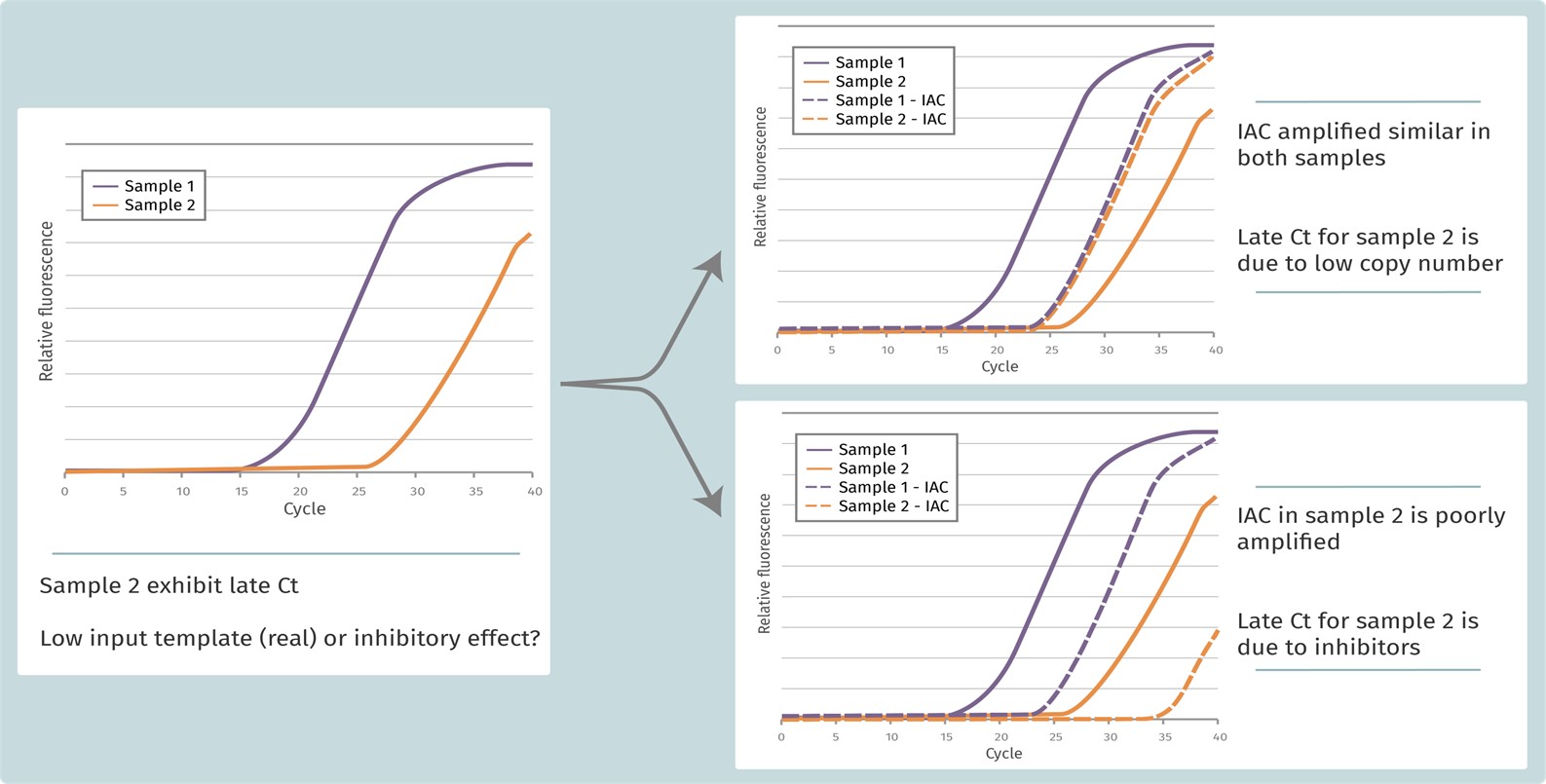
Figure 3. Internal amplification control (IAC) example. Adding an IAC to the reaction is it possible to discriminate if inhibitors are present in the sample.
The KOD concept
Even though numerous methods have been designed to quantify template DNA, very few of them allow simultaneous evaluation of template quantity and quality without the addition of an internal positive control that is co-amplified with the target of interest. Hence Bar and collaborators2 proposed a method called KOD (kinetic outlier detection), based on amplification efficiency calculation for the early detection of non-optimal assay conditions.
KOD approaches compare one or more kinetic parameters from a test reaction to kinetic parameters from a group of reference reactions, preferably ones that have been independently validated. We are not going to dig deep into the mathematical model of KOD, but briefly, this is done comparing qPCR efficiency of a sample (x eff ) with the efficiencies of standard curve samples: z = (x eff - µ eff) / σ eff, where μ eff is the efficiency mean, and σ eff is the standard deviation of the efficiency of standard curve samples. A test sample is classified as an outlier if |z| > 1.96.
In this method, the qPCR efficiency should be estimated in the exponential phase of the reaction. Notably, it has been demonstrated that estimates of qPCR efficiency vary widely according to the approach that has been adopted. For that reason, several versions of the KOD method have been developed, based on a linear or a no-linear regression fitting to the qPCR amplification curve. Being based on the comparison between the test reaction and a reference set, the higher the similarity among reactions, the higher will be the accuracy of the methods. You should consider several parameters on the selection of the reference set: it should comprise replicates based on different concentrations within the expected range, a reference set of 10-15 reactions is usually sufficient to accurately estimate the kinetic parameters, and the composition should be based on comparable kinetics with the studied sample.
It maybe sound complicated, but KOD analysis can be easily fully automated. The standardization of methods to evaluate qPCR efficiency and detect inhibitors in the samples is a critical step required to meet regulatory requirements for evidence-based medicine. If you would like to know more about this topic, have a look on the article from Bar and colleagues3 about validation of kinetics similarity in qPCR.
Conclusion
Many substances present in samples as well as co-extracted contaminants can inhibit your qPCR, compromising template amplification and analysis. If you are working with biological material, this is a big issue.
The gold standard quantification method (Ct method) for real-time PCR assumes that the PCR efficiencies of the compared samples are similar. However, real-time PCR quantification is extremely sensitive to minute variations in PCR efficiency between samples. In fact, after 25 cycles of exponential amplification, a slight variation of 5 % in qPCR efficiency will lead to a three-fold difference in the amount of DNA. Above we review some strategies to assure the accuracy of your qPCR results: to calculate PCR efficiency from a serial dilution, to add internal amplification controls or through detection of kinetic outliers.
We recommend taking those methods in account when you are implementing or optimizing a new protocol for detection of inhibitors in your nucleic acid sample. Furthermore, it is essential to know your sample type and whether it implicates complications during nucleic acids extraction procedure. Always choose the better extraction method to avoid them and test efficiency on your downstream applications.
We know that some sample types are challenging to integrate. If you need support to optimize your workflow, consult Bioecho’s team of experts. They will work with you to develop customized solution that maximize your results.
References
(1) Svec et al. How good is a PCR efficiency estimate: Recommendations for precise and robust qPCR efficiency assessments. Biomolecular Detection and Quantification, 2015. DOI: 10.1016/j.bdq.2015.01.005
(2) Bar et al. Kinetic Outlier Detection (KOD) in real-time PCR. Nucleic Acids Research, 2003. DOI: 10.1093/nar/gng106
(3) Bar et al. (2011). Validation of kinetics similarity in qPCR. Nucleic Acids Research, 2012. DOI: 10.1093/nar/gkr778

Laura is a passionate scientific communicator, with an extensive experience as a researcher in several fields, including human genetics, biotechnology, and neuroscience. Since joining BioEcho in 2022, she enjoys creating appealing content and material for our customers and interested parties. Laura likes practicing yoga, cooking wholesome Mediterranean food, and playing the piano. She also loves spending weekends on the nature, rock climbing and hiking.